


While the above example provides a simple description of how phase transitions can arise in search problems, more realistic models are usually not exactly solvable and one must resort either to simulations or approximate theories. To gain a more intuitive insight into the nature of the transition for constraint satisfaction problems, we examine the search trees for some small cases. Much of the recent work in this area has examined the behavior of the search as a function of the number or tightness of the constraints. Qualitatively, as more constraints are added to a problem, a series of incorrect variable assignments is more likely to violate one of the constraints allowing for earlier pruning. This tends to make the problems easier and can lead to a transition similar to that described above for pruning. However, additional constraints also reduce the number of solutions hence making it more difficult to solve the problem. Thus as constraints are added, these two factors compete against each other. In fact, the loss of solutions is the dominant effect for weakly constrained problems, leading to an increase in typical search cost. This is simply because each new constraint is more likely to eliminate states with many assigned variables (especially solutions, where all variables are assigned) than it is to eliminate states with only a few assignments. For highly constrained problems, on the other hand, the additional pruning becomes dominant leading to a decrease in search cost. This is because the highly constrained problems either have no more solutions to remove, or the remaining solutions are required to exist by the problem specification. In either case, the additional constraints do not remove any more solutions and so the increased pruning is not offset by a further reduction in the number of solutions.
This is easily illustrated with a small graph coloring example. In this problem one is given a graph and required to select, from among a specified set of colors, a color for each node so that nodes linked by an edge have different colors. In this context, each edge in the graph provides a constraint on the allowed colorings. To see the effect of increasing the number of constraints, consider a series of connected graphs constructed from a random tree [43] with 10 nodes (and 9 edges). Additional edges were added randomly to give a series of related graphs. Each graph was then searched using a simple, nonheuristic backtrack search in which nodes were colored in numerical order.
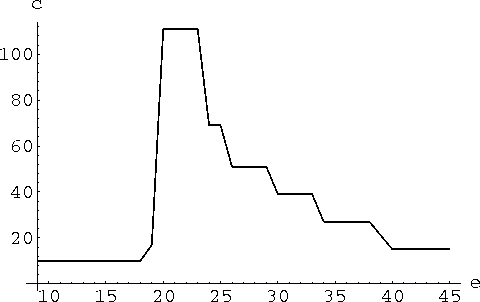
Figure 2: Search cost c to find the first solution, if any, or determine there are none for 3-coloring a randomly generated set of connected graphs with 10 nodes, vs. the number of edges e in the graph. The search used nonheuristic backtrack. The graphs range from a random tree, with 9 edges, to a complete graph (each node linked to every other node) with 45 edges. A solution exists for those cases with 19 or fewer edges. Thus the peak in search cost occurs at the point where the solutions just disappear.
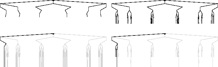
Figure 3: Search trees for coloring some of the graphs. Starting from the upper left and continuing clockwise these correspond to the graphs with 35, 20, 19 and 12 edges respectively. Black lines show the states searched to find the first solution or determine there are none (which is the corresponding search cost shown in Fig. 2). Gray lines show additional consistent partial states that would need to be searched to find all solutions. The direction of the branches indicates the color choice: left, center and right corresponding to colors 1, 2 and 3, respectively. In the cases with at least 20 edges, there are no solutions and the search must examine all consistent assignments with this particular choice of variable ordering before concluding the problem is not soluble.
The resulting search costs, in Fig. 2, show that the sparse and dense graphs are relatively easy to search, while intermediate ones give rise to harder searches. This behavior can be readily understood from the changes in the search trees as edges are added, as shown for a few cases in Fig. 3. With few edges, there are a large number of solutions and one of them is quickly found, without any need for backtracking. As more edges are added, solutions are rapidly eliminated, while partial states with fewer assignments are removed more slowly. This results in a search tree in which many states at intermediate levels do not lead to solutions, increasing the need for backtracking. At some point, the last solutions are eliminated, giving a large increase in the search cost as the backtracking must now continue to check all possibilities. This corresponds to the peak in the search cost found at 20 edges in Fig. 2. At this point we say that the problem is critically constrained in that there are just enough constraints to eliminate the solutions. Beyond this point, additional edges continue to prune the intermediate states in the tree which results in a decreased search cost. This discussion also suggests why the maximum search cost is seen just as the last solutions disappear.
This general observation, relating search behavior to the number of consistent states of various sizes, forms the basis of approximate theories of this transition behavior [56]. In fact this analysis suggests a series of transitions. First, when there are very few constraints, we can expect so many solutions that often one will be found with little or no backtrack, giving a search cost linear in the size of the problem. As more constraints are added, there will be a transition to exponentially large cost, with the rate of exponential growth increasing as more constraints are added, eventually reaching a peak for the critically constrained problems. Beyond this point, the cost grows exponentially, but more slowly. Eventually, for very highly constrained problems, there will be sufficient pruning to make the cost again grow only polynomially. This description applies on average, while the worst case with a given number of constraints can be much harder.
We should note this analysis does not describe, even qualitatively, all the observed behaviors associated with these searches; in particular, the existence of rare but extremely hard searches within the underconstrained regime for many common backtrack search methods [13, 25]. Instead this requires a more careful consideration of the variation in the number of the consistent states actually searched to find the first solution. In the context of Fig. 3, the rare hard cases are due to searches that include a large number of the states indicated in gray.
A peak in the search cost for critically constrained problems is also seen with more sophisticated backtracking strategies as well as for local search methods such as heuristic repair [40], simulated annealing [32] and GSAT [48]. As with the backtracking search described above, small problem examples can also give some intuitive understanding of why these local methods find problems near the transition to be hard [19]. In this case it is due to changes in the proportion of complete assignments that have local improvements.